Building a Machine Learning Stock Trading Bot

Introduction

My favorite class in grad school was Machine Learning for Trading, combining two of my favorite hobbies — coding and stock trading. The class emphasized not to use what we learned in the real world, but it was hard to resist applying the knowledge to potentially make me money (or to lose everything, but what's life without risk).

I primarily used this bot to trade covered calls since it can be a profitable strategy. I started using this strategy manually around the GameStop and AMC phenomenon and decided I wanted to automate the process. I'll cover the tools to create a stock trading bot, the techniques used, the API that facilitated the trades, and share insights with graphs and code snippets — including the parts most tutorials skip: how you actually turn market data into Q-table states, why the reward function is where these projects live or die, and the backtesting traps that make bad strategies look brilliant.

This can be used for any style of trading, but I made mine specifically for covered calls.

Disclaimer

I am not a financial advisor and I made this purely for enjoyment and to see if I could apply my knowledge. I am not trying to beat the market or time it perfectly — I made this to manage my covered calls specifically: to alert me when my calls sell, and, based on history and news, to alert me when it's ideally a good time to buy the stock. Notice the framing: decision support, not autonomous trading. That's a deliberate design choice, not a limitation, and I'd recommend it to anyone building their first bot.

Understanding Options

Before diving deeper, key terms:

• Call Option: a contract giving the buyer the right, but not the obligation, to buy a stock at a specified price (the strike) before a specified date (expiration).
• Put Option: the same, but the right to sell.

A covered call means owning at least 100 shares of a stock and selling a call option against them. You collect the option's premium as income immediately; in exchange, you cap your upside — if the stock rises past the strike, your shares get called away (sold at the strike price). The strategy's profile: it converts potential upside into steady income, performs best in flat-to-slightly-rising markets, and its real risk is the stock falling (the premium only cushions the first few percent of the drop).

The mechanics that any covered-call automation has to reason about:

• Delta roughly maps to the probability the option expires in the money. Selling ~0.30-delta calls — collecting decent premium with a ~70% chance of keeping the shares — is the conventional starting point, and "which delta to sell" is exactly the kind of decision a policy can learn.
• Theta decay is why sellers get paid: option value erodes toward expiration, fastest in the final weeks — which is why selling 30–45 days out and closing early is a common pattern.
• Implied volatility (IV) sets premium size. Selling when IV is elevated relative to its own history (high IV rank) is selling insurance when insurance is expensive — the single most reliable edge in the strategy.

Covered vs. Naked Options

• Covered Call: own the stock, sell the call. If assigned, you deliver shares you already hold. Defined, survivable outcomes.
• Naked Call: sell the call without the stock. If the stock gaps up, losses are theoretically unlimited.

I sell only covered calls to manage risk. Owning the underlying means the worst case is "sold my shares at a price I pre-agreed to" — an outcome you can be mildly annoyed by, not ruined by.

Why Use Q-Learning?

Q-Learning is a reinforcement learning algorithm suited to sequential decision-making problems — like trading, where today's action changes tomorrow's position. Reasons it fits:

• Adaptability: it learns from experience and updates its policy as new data arrives.
• Model-free: it needs no model of market dynamics (good, because nobody has one) — it learns action values directly from interaction.
• Simplicity: a Q-table is transparent. You can read the learned policy — "in state 47, it prefers holding" — which matters enormously when debugging why your bot did something strange with your money.
• Scalability: the framework extends to large state spaces (via function approximation) when the table runs out.

The honest costs: tabular Q-learning needs a lot of experience to converge, and financial markets violate its core assumption cheerfully — the environment is non-stationary (the market of 2021 is not the market of 2019, and a policy learned on one may mislead on the other). This is a real limitation, not a footnote, and it's the deepest reason to keep humans in the loop.

Alternative Models to Consider

I used Q-learning because I learned it in class and was most comfortable with it, but alternatives worth knowing: Policy Gradient methods (REINFORCE, Actor-Critic) that optimize the policy directly and handle continuous action spaces — like position sizing, not just buy/sell; SARSA, Q-learning's on-policy sibling, which learns the value of the policy it actually follows (including its exploration mistakes) and therefore tends toward more conservative policies — arguably a feature in trading; Deep Q-Networks (DQN), replacing the table with a neural network when the state space explodes; LSTMs for sequence prediction as a signal feeding a strategy rather than being the strategy; and genetic algorithms for evolving rule sets. The pragmatic ordering: get the tabular version working first — every lesson it teaches transfers upward, and its failures are legible.

The Plan

1. Data Collection: gather historical stock and options data
2. Feature Engineering: prepare and preprocess the data — and discretize it into states
3. Model Training: train the Q-learner on the historical environment
4. Strategy Implementation: wrap the learned policy in covered-call logic
5. Execution: connect to a trading API (paper account first, always)
6. Evaluation: assess performance against benchmarks that would embarrass it

Tools and Technologies

1. Language: Python
2. ML libraries: NumPy for the Q-learner itself; Scikit-learn/TensorFlow if you graduate to function approximation
3. Data handling: Pandas, NumPy
4. Trading API: Alpaca — commission-free, first-class paper-trading environment
5. Visualization: Matplotlib, Seaborn

Step-by-Step Process

1. Data Collection

Historical data is the environment your Q-learner will live in — price movement and volatility are the "physics" it learns.

import alpaca_trade_api as tradeapi
 
api = tradeapi.REST('APCA-API-KEY-ID', 'APCA-API-SECRET-KEY', base_url='https://paper-api.alpaca.markets')
 
# Fetch historical stock data
stock_data = api.get_barset('AAPL', 'day', limit=1000).df
 
# Fetch options data (use a third-party service if Alpaca doesn't provide options data)
options_data = fetch_options_data('AAPL')

Two data warnings that separate working backtests from fantasy ones. Survivorship bias: if you train only on today's popular tickers, you've trained on companies that didn't fail — history's winners — and the learned optimism doesn't transfer. Options data quality: free options chains are patchy; if the covered-call half of your system is the point, expect this dataset to be the expensive part.

2. Preprocessing Data — and the Step Everyone Skips: Discretization

Normalize prices and compute indicators:

import pandas as pd
 
# Normalize stock prices
stock_data['normalized_close'] = stock_data['close'] / stock_data['close'].iloc[0]
 
# Create state representation (e.g., using moving averages, Bollinger Bands, etc.)
stock_data['SMA'] = stock_data['normalized_close'].rolling(window=20).mean()
stock_data['SMA_ratio'] = stock_data['normalized_close'] / stock_data['SMA']

Here's the part most write-ups hand-wave: a Q-table needs discrete states, and your indicators are continuous. The bridge is binning — divide each indicator's range into buckets (I used quantile-based bins, so each bucket holds equal history rather than equal width), then combine the bucket indices into a single state number:

# Discretize each indicator into 10 quantile bins
stock_data['sma_bin'] = pd.qcut(stock_data['SMA_ratio'], 10, labels=False)
stock_data['bbp_bin'] = pd.qcut(stock_data['BBP'], 10, labels=False)  # Bollinger %B
 
# Combine into one state index: 10 x 10 = 100 states
stock_data['state'] = stock_data['sma_bin'] * 10 + stock_data['bbp_bin']

This design decision is the model. Too few bins and unlike market conditions collapse into the same state (the learner can't distinguish situations that need different actions); too many and each state is visited a handful of times in your whole dataset (the learner never gets enough experience anywhere to learn anything). Two or three indicators at ~10 bins each — hundreds of states against thousands of trading days — is about what tabular learning can feed. If you find yourself wanting five indicators, that's the signal you've outgrown the table and want a DQN.

3. Implementing Q-Learning

The Q-learner maintains a table of expected values for every (state, action) pair, and learns via temporal-difference updates:

import numpy as np
import random
 
class QLearner:
    def __init__(self, num_states, num_actions, alpha, gamma, epsilon, decay_rate):
        self.num_states = num_states
        self.num_actions = num_actions
        self.alpha = alpha  # Learning rate
        self.gamma = gamma  # Discount factor
        self.epsilon = epsilon  # Exploration rate
        self.decay_rate = decay_rate  # Exploration decay rate
        self.Q = np.zeros((num_states, num_actions))
 
    def choose_action(self, state):
        if random.uniform(0, 1) < self.epsilon:
            return random.randint(0, self.num_actions - 1)
        else:
            return np.argmax(self.Q[state, :])
 
    def update_Q(self, state, action, reward, next_state):
        best_next_action = np.argmax(self.Q[next_state, :])
        td_target = reward + self.gamma * self.Q[next_state, best_next_action]
        self.Q[state, action] += self.alpha * (td_target - self.Q[state, action])
        self.epsilon *= self.decay_rate
 
# Initialize Q-Learner
num_states = 100  # must match your discretization: 10 bins x 10 bins
num_actions = 3   # 0 = hold, 1 = buy/write call, 2 = sell/close
learner = QLearner(num_states, num_actions, alpha=0.1, gamma=0.9, epsilon=0.2, decay_rate=0.99)

What the hyperparameters actually control: alpha (learning rate) is how much each new experience overwrites old belief — too high and the table thrashes on noise, too low and training crawls. Gamma (discount factor) sets the planning horizon; 0.9 means rewards ~10 steps out still matter, which is what teaches the learner that holding through a dip can beat panic-selling. Epsilon with decay implements explore-then-exploit: early training tries random actions to discover what works; later training trusts the table. The update_Q line is the entire algorithm — the TD target (reward plus discounted best-next-value) is what the action turned out to be worth; the update nudges the table toward it.

4. Strategy Implementation and the Reward Function

Training iterates through history, simulating actions and updating the table:

# Example of training loop
for epoch in range(100):  # Number of epochs
    state = get_initial_state(stock_data)
    while not done:
        action = learner.choose_action(state)
        next_state, reward, done = take_action(state, action, stock_data)
        learner.update_Q(state, action, reward, next_state)
        state = next_state

The reward function is where I'll be blunt: this is the highest-leverage code in the project, and raw price change is the wrong reward. Reward = price difference teaches the learner to trade constantly (every tick is an opportunity) because it never pays costs. Charge it like reality does:

def compute_reward(action, position, price_change, premium_collected):
    reward = position * price_change          # P&L on the shares
    reward += premium_collected                # income from writing the call
    if action != HOLD:
        reward -= 0.001                        # transaction cost + slippage
    return reward

Even this simple version changes the learned behavior dramatically — with costs charged, the learner discovers that most trades aren't worth making, which is the single truest lesson in retail trading. For the covered-call variant, premium_collected is where the strategy lives: the learner is effectively deciding when writing a call is worth capping the upside, informed by the volatility features in its state. Refinements that matter, in order: penalize drawdowns (risk-adjusted reward, not raw P&L), model assignment when the stock closes above strike, and charge realistic spreads on the options legs — option spreads are much wider than stock spreads, and ignoring them flatters the backtest badly.

5. Testing — Without Fooling Yourself

# Test the trained Q-Learner
test_state = get_initial_state(test_stock_data)
while not done:
    action = learner.choose_action(test_state)
    test_state, reward, done = take_action(test_state, action, test_stock_data)

Backtesting is where trading bots go to look better than they are, so treat these rules as load-bearing. Split time forward: train on 2018–2021, test on 2022–2023 — never shuffle time-series data, and never let the test period leak into any training decision (including your bin boundaries — compute those on training data only, or you've quietly given the model the future). No lookahead: every feature at time t must be computable from data available before t. Freeze exploration at test time (epsilon = 0) — you're evaluating the learned policy, not its dice rolls. And when the test-period results look worse than the training period: that's not a bug, that's the honest number. The gap between the two is your overfitting, measured.

6. Evaluation

Compare against the benchmark that would embarrass the strategy — for covered calls, that's both buy-and-hold and a mechanical covered-call baseline (sell the 30-delta monthly, no intelligence at all). If the learner can't beat the dumb version of its own strategy, the machine learning isn't earning its complexity.

import matplotlib.pyplot as plt
 
# Plot the results
plt.plot(stock_data['date'], stock_data['normalized_close'], label='Stock Price')
plt.plot(stock_data['date'], q_learning_strategy, label='Q-Learning Strategy')
plt.plot(stock_data['date'], buy_and_hold_strategy, label='Buy and Hold Strategy')
plt.legend()
plt.title('Stock Trading Strategy Performance')
plt.xlabel('Date')
plt.ylabel('Normalized Price')
plt.show()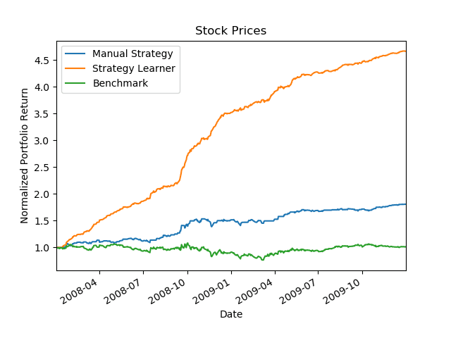

And judge on more than the final portfolio value: Sharpe ratio (return per unit of volatility — the covered-call strategy's smoother ride shows up here even when raw returns tie), maximum drawdown (the worst peak-to-trough loss — the number that determines whether you'd actually keep running the bot), and trade count (a suspiciously active policy is usually a reward-function bug wearing a strategy costume). Then, before any real dollar: paper trade it for months. Alpaca's paper environment exists precisely so your bugs can be free. Mine paper-traded for a full quarter before I let it so much as alert me about real positions.

Conclusion

Creating a machine learning stock trading bot for covered calls spans the full pipeline — data collection, discretization, Q-learning, reward engineering, honest backtesting, and paper-trade validation — and the machine learning turns out to be the easy half. The hard half is epistemological: charging yourself realistic costs, splitting time honestly, benchmarking against the dumb version of your own strategy, and respecting that markets are non-stationary in a way that flatters every backtest. Build it anyway — as decision support with a human on the trigger, it's one of the best end-to-end ML projects you can do, and every trap it teaches you to avoid is a trap that shows up in production ML far from finance. Happy (careful) trading!